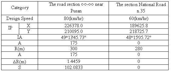
ESTIMATION OF THE DESIGN ELEMENTS OF HORIZONTAL ALIGNMENT BY THE METHOD OF LEAST SQUARESJongchool LEE, Junghoon SEO and Jongho HEO, KoreaKey words: AbstractIn this study, the road linear shape was sampled by using the centerline path, the design elements of horizontal alignment were deduced by applying the Method of Least Squares, and the accuracy was analyzed. By this method, IP, IA, R, ΔR and A-parameter were also determined. By observing relatively long straight sections, the approximate values could be estimated, and particularly, the considerably accurate value of A-parameter was determined. This study, using the Method of Least Squares, aims to contribute to the development of the alignment examination in frequent traffic accident regions. 1. INTRODUCTIONKorea is a small country with relatively large mountainous areas and has many difficulties from planning to completing one road. Maintaining a completed road presents even more difficulties. Presently, in estimating design elements, the result varies according to the engineer and there are many cases that question the reliability of the results. Therefore, this study aims to sample the road linear shape using the centerline path, to deduce the design elements of horizontal alignment applying the Method of Least Squares, and to analyze the accuracy. 2. METHOD OF LEAST SQUARES FOR SAMPLING LINEAR SHAPEIt must first be decided how to use the sample observation value. As the sample observation value is not on a perfectly straight line, several different kinds of straight lines can be drawn through the displayed data. The line, which explains the data most appropriately, must be selected. It is necessary to define which the most appropriate line is, to avoid subjective judgment in finding the sample regression line. It is logical to define the straight line, which has the smallest residual on the average as the most appropriate. The problem accompanied by this method is that though any residual never approaches 0 some residuals become plus and others become minus the sum of the residuals is always 0. To avoid this problem, the straight line that has the smallest sum of squares of residuals is defined as the most appropriate line. This process is called the Method of Least Squares. The Method of Least Squares is to deduce a straight line that minimizes the sum of squares of the distance from the observed datum to the straight line. 3. DATA COLLECTION AND ARRANGEMENT3.1 Selection of Investigation AreaTable 3.1. Horizontal Design of Investigation Area
The road extension section near Pusan and parts of curved section in, National Road n.35 were selected for investigation. The road near Pusan is in the finishing stage, and the National Road n.35 is expanded into a four-lane road both ways and has relatively fine horizontal alignment. 3.2 Data Collection And Arrangement3.2.1 Elements of Observation Equipments The elements of observation equipments are shown in <Table 3.2.1>. Table 3.2.1 Elements of GPS Equipment
3.2.2 Collection of Observation Data The chain distance was established and the center line path was measured by the KINEMATIC Method of GPS Measuring Method in the road extension section near Pusan and parts of curved section in, National Road n.35. The chain distance was about 5m in the straight line section, the data acquisition interval according to the chain distance was set on the basis of 3 seconds, and the data reception interval was on the basis of 24 seconds. 3.2.3 Data Calculation Method In the data observed by point, the centerline path was calculated through indoor GPS post-management process, and the details are as follows. 1) Straight Line Path
Figure 3.2.1 Observation Point within Straight-line Section And Regression Line 2) Circular Curve Path
Figure 3.2.2 R And the Center Point of Circular Curve The minimum length of prescribed horizontal curve is set twice as long as the minimum transition section length. That is, the minimum horizontal length can be satisfied only with the transition curve, but in this case, it cannot be regarded as smooth handling, because the driver must hurriedly turn the steering wheel although the length condition to give a satisfactory curve was satisfied. Besides, as it is viewed as bent if sufficient attention is not paid to the establishment of superelevation, the curve does not give a smooth feeling to the driver. Therefore, it is desirable to insert a circular curve with some extents of length between these two transition curves. The analysis flow chart for finding value R in the circular curve section is shown in <Figure 3.2.3>.
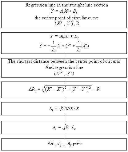
Figure 3.2.3. R-Analysis Flow Chart As the center of circular curve is on the isometric line, the value R with the smallest SSE (Sum of Squares Error) and the center coordinates of circular curve was found by moving the center point of the circular curve by 10cm with IP coordinates as a starting point. The program [1,2] was set to input the coordinates within the circular curve section, the isometric line of the two transition lines, and the IP coordinates in the following picture. In this study, R and the center point of circular curve were calculated by measuring the road center point within the circular curve section through a field investigation. 3) Clothoid Curve In this study, A-parameter was found using the transition curve shift of Clothoid curve in <Figure 4.2.4>. The analysis flow chart is shown in <Figure 3.2.5>. A shift is the extent to which the center of the circular curve was moved inward, when it is accessed directly to the circular curve from the straight line section without inserting a transition curve and when the transition curve is inserted into its interval. In other words, it means that the difference between the shortest distance between the straight line and the center point of transition line, and R.
Figure 3.2.4 In this study, a shift was regarded as the difference between the shortest distance between the center point of circular curve and regression line, and R. And a shift(ΔS), transition curve length and A Transition Curve Shift were found using the value R found in the above, the center coordinates of circular curve and the regression line.
Figure 3.2.5. A-Analysis Flow Chart 4. ANALYSIS OF HORIZONTAL ALIGNMENT PATH4.1 Section near Pusan
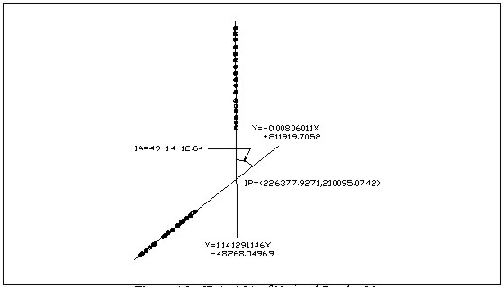
Figure 4.1. IP And IA near Pusan The vertical distance is about 80~90m and the chain distance is about 10m in the straight line section of road extension section near Pusan. The regression equation is as follows.
The center part of the circular curve section was found by dividing the distance between the two first points which miss the maximum residual in the straight line section in a ratio of 1 : 2 : 1. The value R was gained while moving the center point of the circular curve from IP-point and appreciated with the SSE of each point. The SSE has the minimum value of 0.125 in the point that the distance from IP-point becomes 310.5m. The center point, the value R, and the vertical residual of each point are shown in <Figure 4.2>.
Figure 4.2 Vertical Residual 4.3 Section, National Road n.35
Figure 4.3. IP And IA of National Road n.35 The vertical distance is about 260-380m and the chain distance is about 20m in the section of National Road n.35. The regression equation is as follows.
The center part of the circular curve section was found by dividing the distance between the two first points which miss the maximum residual in the straight line section in a ratio of 1 : 2 : 1. The value R was gained while moving the center point of the circular curve from IP-point and appreciated with the SSE of each point.
Figure 4.4 Vertical Residual 4.3 Comparison and Analysis with the Execution Drawing
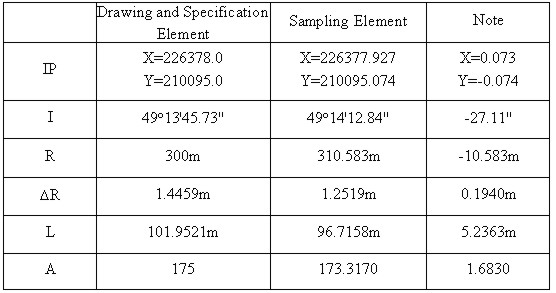
Table 4.3.1 Sampling Element in the Section near Pusan
Table 4.3.2 Sampling Element in the ??-?? Section of National Road n.35 5. CONCLUSIONIn this paper, the horizontal design elements were estimated by the method of statistical inference, and its results are summarized as follows.
REFERENCES
CONTACTProf. Jongchool Lee Junghoon Seo Jongho Heo 20 April 2001 This page is maintained by the FIG Office. Last revised on 15-03-16. |


